Final Group Report
Mice Preoptic Hypothalamus — Interactive Visualization Dashboard Project
Project Milestone 3: Report Section
Overview
This project investigates how neuronal gene expression varies across spatial regions, cell clusters, behaviors, and sexes in the hypothalamic preoptic area of mice. Using MERFISH data, we focus on key genes (e.g., Fos, Gal, Th, Bdnf, Adcyap1, Esr1, Oxtr, Gnrh1, Slc17a6, Gad1) and examine patterns across Excitatory, Inhibitory, and Ambiguous neuronal classes. The analyses combine spatial mapping, cluster-level comparisons, and sex-stratified gene expression to highlight heterogeneity, sex dimorphism, and behavior-driven activation. Visualizations are designed to clarify these patterns, allowing researchers to identify key clusters, co-expression networks, and extreme gene expressors in different conditions.
Audience
This report is intended for neuroscientists, computational biologists, and behavioral researchers who are interested in single-cell gene expression dynamics in the hypothalamus. It is also useful for lab members or students seeking insights into sex- and behavior-specific activation patterns, spatial cluster organization, and the functional role of key neuromodulators.
Dataset
The dataset includes approximately 50,000 neurons across multiple mice, annotated with behavior (Naïve, Parenting, Mating, Aggression), biological sex, Bregma slice, cell class, cluster ID, and expression for 155–160 genes. Cells were filtered to focus on neuronal populations, and key genes were selected based on relevance to social behavior, hormone signaling, and neural activity. Preprocessing included downsampling for computational efficiency, normalization, and exclusion of non-neuronal cells.
General Takeaways
From this dataset, the audience should be able to explore patterns of neuronal heterogeneity across behaviors, sexes, and spatial locations. Key findings include behavior-driven activation (e.g., Fos upregulation during Parenting/Mating/Aggression), sex-specific expression of hormone receptors (Esr1, Oxtr), and co-expression networks among neuromodulatory genes (Gal, Th, Bdnf, Adcyap1). Visualizations allow identification of cluster-specific activation, spatial segregation of sex-biased circuits, and extreme gene expressors. Overall, the analyses reveal how neuronal populations dynamically encode social behavior, emphasizing sex differences and functional specialization in hypothalamic circuits.
Team Member I: Prateek
Theme
Quantifying Sources of Variation: The primary focus is to distinguish gene expression differences attributable to biological sex from those caused by individual animal-to-animal variability (batch effects).
View I: Variance Decomposition Overview
Title: Splitting the Differences: Sex vs. Animal ID Variance
Analytic Questions and Tasks: For the most abundant neuronal clusters, what percentage of the total gene expression variability is explained by Animal Sex versus Animal ID? - Retrieve Value: Obtain the precise percentage of variance ($\eta^2$) for specific genes. - Filter: Focus the analysis on specific, high-abundance neuronal clusters. - Find Extremum: Identify genes exhibiting the strongest sex-driven or ID-driven variance.
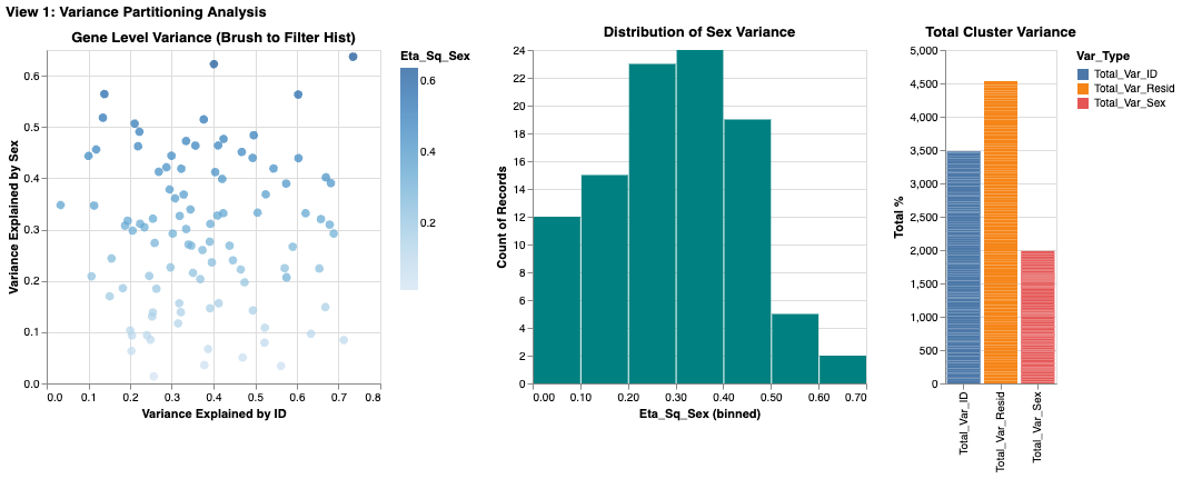
Suitability of Visualization: The multi-view approach is highly effective. The scatter plot allows for the simultaneous comparison of two quantitative variables ($\eta^2_{Sex}$ vs. $\eta^2_{ID}$), making it easy to find extremes (genes far from the diagonal). The stacked bar chart complements this by showing the part-to-whole relationship of the variance components for the filtered cluster.
View Description & Channels: A dashboard with three coordinated views: a gene-level scatter plot (left) showing $\eta^2_{Sex}$ vs. $\eta^2_{ID}$, a histogram of variance distribution (middle), and a normalized stacked bar chart (right) showing the aggregate variance for the selected cluster. - Marks: Points for individual genes in the scatter plot; Bars for aggregated data in the histogram and stacked bar chart. - Channels: - Position (Spatial): On the scatter plot, the horizontal position encodes $\eta^2_{ID}$ and vertical position encodes $\eta^2_{Sex}$. This uses spatial separation to allow for rapid comparison of the two factors. - Length/Height: In the bar charts, length encodes the quantitative proportion of variance. - Color (Nominal): In the stacked bar chart, distinct hues differentiate the variance sources ("Sex" vs. "ID").
Interaction: - Dropdown Selection (Filtering): A dropdown menu allows the user to filter the entire dashboard by Neuronal Cluster, reducing visual clutter and focusing the analysis. - Slider (Filtering): A slider filters genes based on a minimum $\eta^2_{Sex}$ threshold, allowing the user to remove low-variance "noise" and focus on significant markers. - Brush & Link (Cross-Filtering): An interval selection (brush) on the scatter plot is linked to the other views. Selecting a group of genes in the scatter plot filters the histogram and highlights their aggregate contribution in the stacked bar chart, providing immediate visual feedback on their distribution.
Critique: This view effectively separates global patterns from gene-level specifics. The scatter plot's spatial encoding is excellent for spotting correlations and outliers. However, the primary limitation is occlusion in the scatter plot due to the large number of genes, making individual points hard to resolve in dense areas. While the slider helps mitigate this by filtering, future iterations could explore density-based visualizations (like hexagonal binning) to better represent crowded regions.
View II: Confounding Effect Analysis
Title: Impact of Batch Correction on Sex Differences
Analytic Questions and Tasks: Are there genes with large apparent sex differences that are significantly reduced when correcting for individual animal effects? - Compare: Directly contrast the Original Log-Fold Change (LFC) with the Corrected LFC for each gene. - Compute/Assess: Evaluate the magnitude of the "correction shift" (the residual difference).
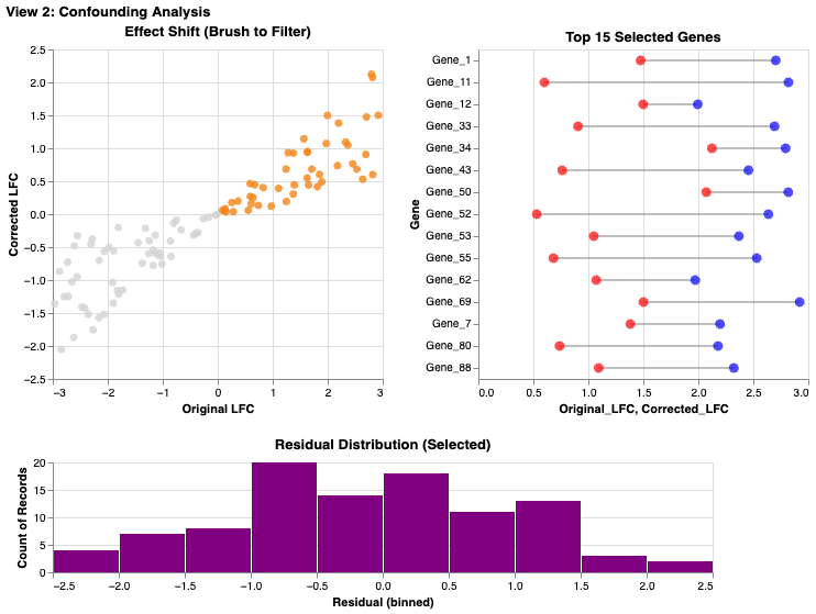
Suitability of Visualization: The lollipop plot is an ideal choice for this comparison task. The explicit line connecting the "Original" and "Corrected" points for each gene provides a stronger perceptual cue for evaluating change than side-by-side bars would.
View Description & Channels: A dashboard featuring a scatter plot of Original vs. Corrected LFC (left) linked to a lollipop plot highlighting top genes (right), with a histogram of residuals below. - Marks: Points and Lines form the lollipop glyphs, explicitly linking the two states of a single gene. Points are used in the scatter plot. Bars in histogram. - Channels: - Length (Delta): The length of the lollipop stick visually encodes the magnitude of the batch effect correction. - Color (Nominal): Red and blue denote the "Original" and "Corrected" states, respectively. - Position relative to Identity Line: In the scatter plot, a point's distance from the $y=x$ diagonal indicates the degree of correction.
Interaction: - Brush & Link (Cross-Filtering): An interval selection on the global scatter plot filters the lollipop plot to show only the selected genes, allowing users to drill down from the overview to specific examples. - Radio Button (Sorting/Encoding): A radio button allows the user to re-sort the lollipop plot (e.g., by original LFC or by correction magnitude), facilitating different comparison tasks.
Critique: The lollipop plot is highly effective for the compare task, leveraging the Gestalt principle of connectivity to show the shift in values. A potential downside is that the global scatter plot relies on interpreting distance from the diagonal, which can be less intuitive for some users than direct comparison. Adding the histogram of residuals helps by providing a clear summary of the distribution of correction magnitudes.
View III: Robustness Check
Title: Biological Consistency Across Animals
Analytic Questions and Tasks: Is the observed sex difference for a given gene consistent across all animals, or is it driven by a few outliers? - Characterize Distribution: Assess the spread and central tendency of gene expression across individual cells and animals. - Find Anomalies (Outliers): Identify individual animals or cells that deviate significantly from the group pattern.
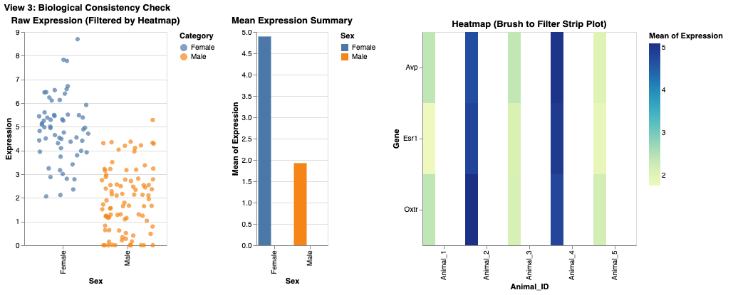
Suitability of Visualization: A jittered strip plot is superior to a box plot for this task because it displays the raw data points. This reveals the true sample size, underlying distribution, and presence of distinct subpopulations, which summary statistics (like quartiles in a box plot) can hide.
View Description & Channels: A dashboard combining a jittered strip plot (left), a mean bar chart with error bars (middle), and a sample-level heatmap (right). - Marks: Points for individual cells in the strip plot; Bars for means. - Channels: - Position (Y-axis): Encodes the quantitative gene expression level. - Color (Nominal): Points are colored by `Animal_ID`, allowing for rapid identification of data from specific individuals. - Spatial Jitter: Random horizontal displacement is added to points to reduce occlusion and reveal local density.
Interaction: - Dropdown Selection (Parameterization): Users select a specific gene (e.g., *Esr1*, *Oxtr*) from a dropdown, which updates all views to show data for that gene. - Cross-Filtering: Selecting specific animals in the heatmap filters the strip plot to show only cells from those individuals, enabling focused comparison.
Critique: This view prioritizes transparency over summarization. By showing every cell as a point, it avoids the potential ecological fallacies of aggregated data. Coloring by `Animal_ID` is highly effective for the find anomalies task. The main limitation is scalability; with a very large number of cells, the strip plot can become cluttered. The cross-filtering capability from the heatmap is a crucial feature that mitigates this by allowing users to zoom in on subsets of the data.
Individual Summary
My analysis focused on disentangling biological sex differences from technical batch effects (Animal ID). I structured my approach in three stages: a high-level variance decomposition (View I), a direct evaluation of the correction method (View II), and a granular robustness check at the individual animal level (View III).
A key realization was that while summary statistics (like those in View I's bar charts) are useful for general trends, they often obscure crucial underlying distributions. This motivated the design of View III, where I chose a jittered strip plot over a standard box plot. This decision was critical for assessing whether a "sex difference" was a consistent biological phenomenon across animals or an artifact driven by outliers.
A significant challenge was managing visual complexity in crowded plots. In View I, the gene-level scatter plot suffered from severe occlusion. While interaction (filtering/brushing) helped, a static solution like density binning might have been more effective for the overview. However, the "lollipop" design in View II proved highly successful, offering a clearer visual representation of change than alternative designs like grouped bar charts. Ultimately, this suite of visualization tools enables a user to not only identify potential sex-linked genes but to rigorously evaluate the reliability and robustness of those signals against confounding noise.
Team Member II: Alina Hameed
Theme
Spatial Organization and Molecular Identity of Neural Cell
Classes
The primary focus is to understand how different neural cell classes are
distributed across brain regions and how molecular features—particularly
Gad1 expression—distinguish neuronal subtypes. The
central question is how spatial location relates to molecular identity,
and whether gene expression patterns validate or refine cell class
definitions.
View I: Brain Cell Atlas Dashboard
Title
Spatial Distribution and Regional Composition Across Brain Slices
Analytic Questions and Tasks
Where are different cell classes located in the brain, and how does their distribution change across the anterior–posterior axis?
Locate: Identify where specific cell classes (Excitatory, Inhibitory, Glia, Vasculature, Ependymal, Other) appear in anatomical space.
Characterize Distribution: Examine how each cell class is distributed along the Y-axis using ridge plots.
Compare: Contrast cell class composition across bregma slices.
Distinguish: Differentiate cell classes based on spatial organization.
Summarize: Aggregate cell counts by class and slice to reveal compositional trends.
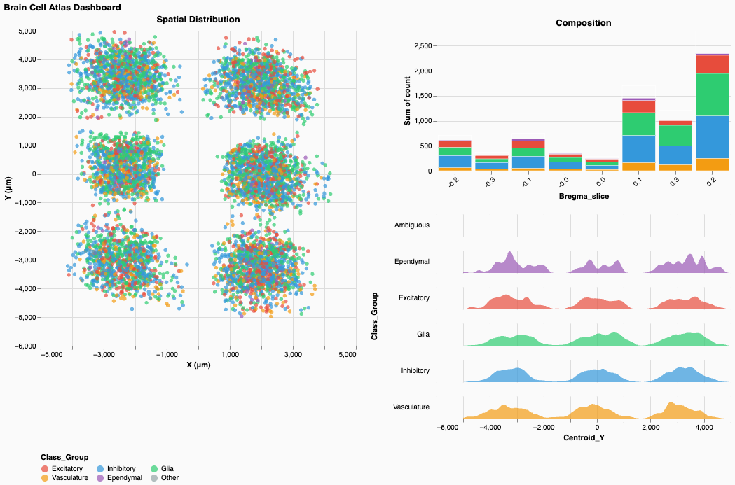
Suitability of Visualization
The multi-view structure is highly effective for connecting single-cell data to global spatial patterns. The spatial scatter plot provides direct mapping to anatomical coordinates, revealing six distinct tissue sections arranged in a grid. The ridge plots reveal how cell classes segregate along the Y-axis, while the stacked bar chart summarizes global composition by slice. Together, these views enable both fine-grained and high-level spatial reasoning.
View Description & Channels
A coordinated dashboard with three views arranged as:
(Spatial Scatter | Composition Bar Chart & Ridge
Plots)
- Left: Spatial scatter plot of all cells by centroid
X and Y
- Right–Top: Stacked bar chart showing class
composition across bregma slices
- Right–Bottom: Ridge plots showing Y-axis density by cell class
Marks:
Points for cells, area marks for ridgelines, stacked bars for
composition.
Channels:
- Position (Spatial): X and Y encode true anatomical
coordinates.
- Color (Nominal): Cell class is encoded consistently
across all views:
- Red/Coral: Excitatory
- Blue: Inhibitory
- Green: Glia
- Orange: Vasculature
- Purple: Ependymal
- Red/Coral: Excitatory
- Area/Width: In ridge plots, width encodes
density.
- Length: In stacked bars, height encodes cell count.
Interaction
- Brush & Link (Cross-filtering): Selecting cells in
the spatial plot updates ridge plots and composition bars.
- Legend Filtering: Clicking class labels filters all
views.
- Hover (Details-on-Demand): Tooltips show
coordinates, class, and metadata.
- Click Selection: Selecting bars or ridge regions highlights spatial locations.
Critique
This view supports multi-scale analysis from individual cells to tissue-wide composition. Color consistency effectively reduces cognitive load, and ridge plots clearly reveal that Ependymal cells cluster at low Y-values (ventral regions), while others overlap more centrally. However, severe occlusion in the spatial plot makes local density hard to interpret. Density overlays or hexagonal binning would substantially improve readability. Additionally, the use of absolute counts in the composition chart limits cross-slice comparison; normalized (100%) bars would better convey relative structure.
View II: Gene Co-expression Explorer
Title
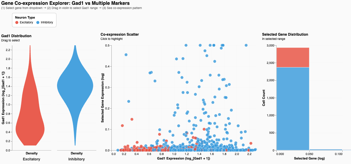
Gad1 Co-expression Explorer: Neuron Type Validation Through Molecular Signatures
Analytic Questions and Tasks
How does Gad1 expression distinguish Excitatory and Inhibitory neurons, and how does it relate to other marker genes?
Compare: Contrast Gad1 distributions.
Correlate: Examine relationships between Gad1 and selected genes (e.g., Sst).
Filter: Brush Gad1 ranges to isolate subpopulations.
Retrieve Value: Access individual cell expression values.
Find Extremum: Identify extreme expressers.
Suitability of Visualization
The violin plot exposes full distribution shape, validating the molecular distinction between cell types. The scatter plot shows co-expression patterns at the single-cell level, and the stacked bar summarizes cell type composition in the selected Gad1 range. This triad effectively links univariate, bivariate, and aggregate analysis.
View Description & Channels
A dashboard with three linked views arranged as:
(Violin Plot | Co-expression Scatter | Summary Bar
Chart)
- Violin: Gad1 distribution by neuron type
- Scatter: Gad1 vs. chosen marker gene
- Bar Chart: Class composition for brushed range
Marks:
Area for violins, points for scatter, bars for composition.
Channels:
- Position (Quantitative):
- Gad1 mapped to violin Y-axis and scatter X-axis
- Marker gene mapped to scatter Y-axis
- Gad1 mapped to violin Y-axis and scatter X-axis
- Width: Density in violins
- Color: Neuron class (Red = Excitatory, Blue =
Inhibitory)
- Length: Cell count in bars
Interaction
- Dropdown (Parameterization): Select marker gene for
scatter Y-axis.
- Brush (Filtering): Select Gad1 range directly on
the violin.
- Cross-linking: Selection highlights corresponding
cells and updates counts.
- Tooltips: Display precise expression values.
Critique
The violin plot clearly demonstrates non-overlapping Gad1 distributions, providing strong biological validation of cell classes. The scatter plot reveals heterogeneity among inhibitory neurons, particularly in Sst expression. However, overplotting in dense regions reduces interpretability. Statistical summaries such as correlation coefficients and reference thresholds would further strengthen analytical rigor. The right panel title is also misleading—it summarizes class composition, not gene distribution.
Individual Summary
My work focused on linking spatial organization (View I) and molecular identity (View II) to characterize neural cell classes. This reflects a core neuroscience principle: neuronal identity arises from both anatomical context and gene expression.
A major design choice was using violin plots instead of box plots in View II. This revealed the complete separation of Gad1 expression between Excitatory and Inhibitory neurons—an essential biological insight that summary statistics would obscure. Similarly, I intentionally showed individual cells in View I to avoid masking heterogeneity, even though this introduced severe occlusion.
The central challenge was overplotting. Alpha transparency was insufficient, and in retrospect I should have implemented density-based representations for overview with semantic zoom to reveal individual points at higher resolution. Despite this, maintaining consistent color encoding across views enabled intuitive cross-view tracing of cell classes.
With further iteration, I would:
- Add adaptive density rendering
- Include statistical summaries (correlation coefficients, confidence
intervals)
- Normalize composition charts
- Integrate spatial origin into molecular views
- Add biologically meaningful reference annotations
Together, these improvements would better balance expressiveness with efficiency—supporting both exploratory insight and confirmatory analysis.
Team Member III: Emily
View I — Sex-Biased Activation Across Behaviors (Heatmap + Linked Bar Chart)
Sex-Biased Activation Across Behavioral Conditions
Questions and Low-Level Tasks
Analytic Question:
Do male and female mice activate the same neuronal clusters during parenting, mating, and aggression, or are there sex-specific activation patterns?
Low-Level Tasks (Stasko taxonomy):
- Filter: Select a specific sex-bias metric to
re-encode the heatmap.
- Compare: Compare female vs. male activation per
cluster × behavior.
- Characterize Distribution: Examine how sex bias
varies across behaviors and clusters.
- Find Anomalies: Identify unusually biased
clusters or conditions.
- Details-on-demand: View exact activation counts for a selected cluster–behavior pair.
View (Visualization)
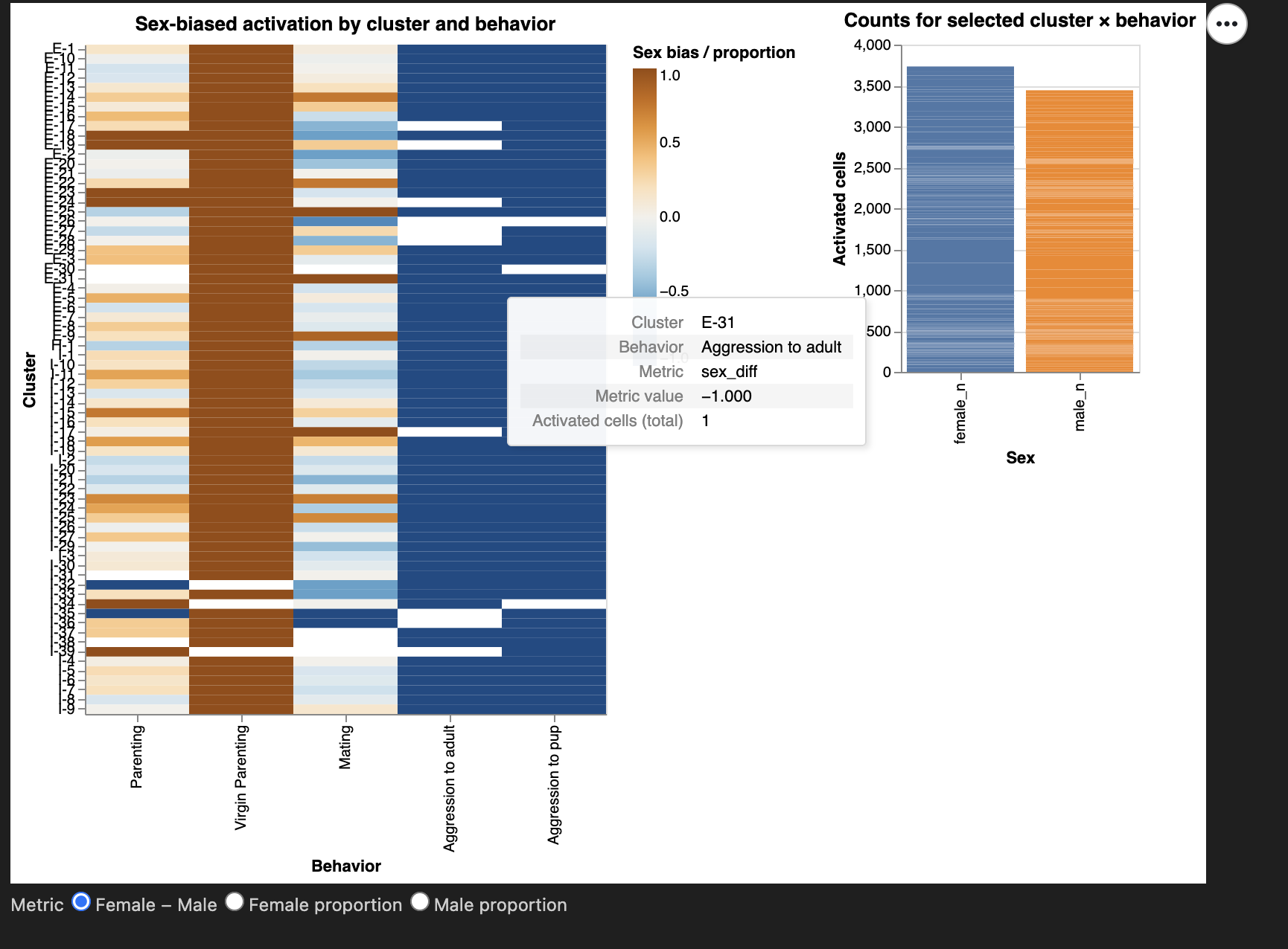
This view consists of an interactive heatmap paired
with a linked bar chart.
The heatmap displays activation of neuronal clusters across behavioral
conditions, with rows representing Neuron_cluster_ID and
columns representing Behavior. Each cell encodes the
sex-bias of activated cells using a diverging color
scale.
Above the heatmap, I include a radio-button widget that allows the user to switch between three metrics:
- Female − Male difference
- Female proportion
- Male proportion
Clicking a heatmap cell triggers a linked bar chart
to the right, which shows the exact female_n and
male_n activated cell counts for that cluster–behavior
pair.
This two-part design supports: - global pattern
identification (via heatmap)
- precise numerical inspection (via bar chart)
Describe the Visualization and Characteristics of Channels
Marks
- Rectangles (heatmap cells)
- Bars (counts of activated cells)
Channels
Color (diverging, blue–orange)
- Encodes sex bias (
sex_diff,female_prop, ormale_prop).
- A diverging palette is appropriate because sex_diff has a meaningful zero point, making polarity between male- and female-biased activation intuitive.
Position (x-axis)
- Encodes Behavior in a consistent left-to-right
order (Naive → Parenting → Aggression).
- Supports conceptual comparison.
Position (y-axis)
- Encodes Neuron_cluster_ID.
- Vertical grouping supports scanning across behaviors.
Length (bar chart)
- Encodes magnitude of female vs male activated cell counts.
Why these choices?
Sex-based comparative analysis benefits from: - fast global
pattern detection → best handled by color in a
matrix
- precise quantitative lookup → best handled by
bar charts
This aligns with course visualization principles:
Use strong perceptual channels (color, position) for pattern recognition
and length for quantitative precision.
Describe the Interaction and Characteristics of Interaction
IMI Interaction — Metric Radio Buttons
Implemented using an alt.param.
Users toggle among three encodings of sex bias.
Supports tasks: - Filter: switches the
displayed metric
- Compare: examine male vs female activation under different
definitions
Why:
Different metrics highlight different aspects of sex bias.
Giving users control avoids relying on a single potentially misleading
encoding.
DMI Interaction — Click Selection on Heatmap (Linked View)
Implemented with selection_point.
Clicking a heatmap cell updates the bar chart with exact counts.
Supports tasks: - Compare: directly compare
sexes numerically
- Find Anomalies: check if extreme colors arise from small or
large counts
- Details-on-demand: exact values displayed
Why:
Color alone lacks precision; the bar chart provides necessary numerical
detail.
Hover Tooltips
Provide: - Cluster ID
- Behavior
- Metric name
- Metric value
- Total activated count
Supports tasks:
Details-on-demand, Characterize Distribution
Critique of the View
What works well
- The heatmap clearly shows global sex-bias patterns.
- The metric radio buttons allow flexible biological
interpretation.
- The linked bar chart grounds color impressions in actual
counts.
- Consistent behavior ordering supports cross-view comparison.
What could be improved
- Small-count clusters may mislead; a minimum-count slider (planned
for PM4) would help.
- Heatmap height grows with cluster count; collapsible cluster groups
could help.
- Adding confidence intervals could contextualize large sex differences.
Suitability for the Tasks
This view directly answers the analytic question and fully supports
the required low-level tasks.
The combination of: - high-level pattern visualization
(heatmap)
- interactive detail view (bar chart)
enables exploration and interpretation grounded in the data.
Overall, I think this is a strong and effective visualization aligned with analytical goals and course principles.
View II — Spatial Segregation of Sex-Biased Behavior Circuits
Spatial Distribution and Anatomical Segregation of Sex-Biased Activated Neurons
Questions and Low-Level Tasks
Analytic Question 2:
Are sex-biased behaviorally activated neurons spatially segregated within the preoptic region?
Low-Level Tasks (Stasko taxonomy):
- Locate: Identify where activated neurons lie in
(X, Y) anatomical space.
- Cluster: Detect visually coherent spatial
clusters enriched for each sex.
- Compare: Contrast spatial patterns for male vs
female neurons across behaviors.
- Summarize: Examine sex bias aggregated within
anatomical subregions (Bregma bins).
- Filter: Adjust which subset of neurons is
displayed by selecting a behavior.
- Details-on-demand: Hover to inspect local anatomical and gene-expression details.
All tasks relate directly to investigating spatial segregation of functional circuits.
View (Description)
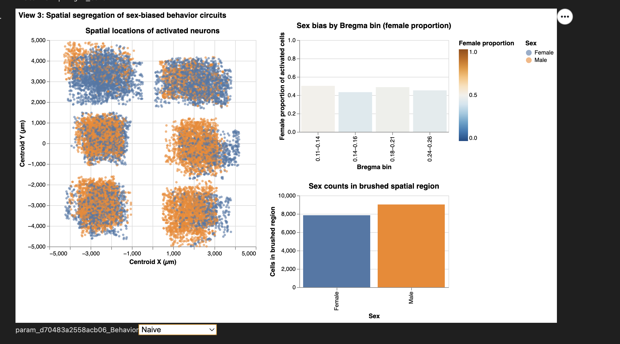
This view is composed of three coordinated visualizations, arranged to allow users to explore anatomical segregation from whole-region patterns down to specific local subregions:
- Spatial scatterplot of activated neurons in
Centroid_X × Centroid_Y space, colored and shaped by sex.
- Provides the main spatial map of where neurons lie in the preoptic region.
- Sex bias by Bregma bin (female proportion per
anatomical slice).
- Each bin acts as a coarse anatomical proxy, showing which subregions are predominantly male- or female-biased.
- Sex counts within a brushed spatial region.
- Brushing on the scatterplot updates this panel with the local sex ratio inside the selected anatomical area.
Coordinated Interactions: - A behavior
dropdown filters all three visualizations simultaneously
(IMI).
- A spatial brush on the scatter links to Viz 3
(DMI).
- A bar-chart click on Bregma bins highlights
corresponding neurons in Viz 1 (DMI).
Together, the three views form a powerful exploratory tool directly supporting the spatial segregation question.
Describe the Visualization and Characteristics of Channels
Marks
- Circles — activated neurons in anatomical space
- Bars — Bregma-bin summaries and brushed-region summaries
Channels
Position (X and Y)
- Encodes anatomical coordinates (Centroid_X,
Centroid_Y).
- This is the strongest perceptual channel and essential for spatial tasks.
Color (categorical)
- Encodes sex (Male/Female).
Color (quantitative, diverging)
- Encodes female proportion across Bregma bins.
- Immediately distinguishes female-biased vs male-biased slices.
Shape
- Reinforces sex encoding, improving accessibility (e.g., colorblind users).
Length (bar height)
- Shows either (1) female proportion or (2) raw counts in brushed regions.
Why these choices?
- Spatial tasks → position
- Sex differences → color + shape
- Bias interpretation → diverging colormap
- Summaries → bar height for clarity
These decisions directly follow principles from class and support the analytical goals.
Describe the Interaction and Characteristics of Interactivity
IMI #1 — Behavior Dropdown
Users select one of the six behavioral conditions.
All visualizations update in sync.
Tasks supported: Filter, Compare
Why: Different behaviors activate different neural
circuits; segregation may be behavior-specific.
DMI #1 — Spatial Brush on Scatterplot (Bi-directional Link)
A rectangular brush selects any XY region of the brain.
The “Sex counts in brushed region” panel updates automatically.
Tasks supported: Locate, Cluster, Summarize
Why: Allows the user to test hypotheses about
microanatomical pockets enriched for one sex.
This is a meaningful analytic interaction because it converts local anatomical selection into quantitative evidence.
DMI #2 — Click Selection on Bregma Bins
Clicking a bar highlights only the neurons from that bin in the scatterplot.
Tasks supported: Locate, Compare
Why: Connects coarse anatomical slices to precise XY
spatial locations, revealing whether certain slices house the strongest
sex biases.
Additional Hover Interaction
Tooltips show each neuron’s: - XY coordinates
- Sex
- Bregma value
- Fos expression
Tasks supported:
Details-on-demand
Critique of the View
What Works Well
- The scatterplot effectively reveals spatial segregation or overlap
between male and female activation.
- The Bregma-bin chart gives an intuitive anatomical summary of sex
bias.
- Bi-directional interactions promote meaningful exploration rather
than passive viewing.
- Behavior filtering isolates condition-specific activation
patterns.
- Encoding choices remain consistent with Views I and II, supporting dashboard coherence.
Areas for Improvement
- Dense XY regions may obscure subtle sex differences; optional
jitter or density contours could help.
- Bregma bins are anatomical approximations; more precise nuclei-level
metadata would enable finer summaries.
- Small brush selections may be difficult for some users; zoom functionality could enhance control.
Suitability for the Task
This view directly addresses spatial segregation by integrating: -
3 coordinated visualizations,
- 2 IMI interactions,
- 2 DMI interactions, and
- clear encodings of both sex and anatomical
position.
It fully supports all low-level tasks and provides a clear pathway to answering the high-level analytic question of whether sex-biased behaviorally activated neurons segregate anatomically within the preoptic region.
Team Member IV: Vincy
Some advanced data wrangling
Wrangling beyond the basics was necessary for my planned views, I applied some purposeful preprocessing steps as follows to make the dashboard rendering more computationally manageable and easier for interpretation:
Further downsampling
Randomly selected ~10,000 cells while preserving original proportions of Cell_class, Animal_sex, Behavior, and Bregma level (originally 1 milion, previously trimmed to ~80,000 for basic EDA).
This reduced memory use significantly and enabled real-time bidirectional brushing/linking without sacrificing statistical representation.
Behaviour label refinement
I found the original behavior annotations sometimes too ambiguous. Using prior exploratory analysis, I renamed:
- “Aggression to pup” →”Pup-directed male aggression”.
Only male mice showed infanticide (killing of newborn mice) in this dataset.
- “Naive” →”Naive home-cage (control)”
To better emphasize the undisturbed baseline condition.
- “Aggression to adult”: “Male–male aggression”
To clarify ‘aggression mice’ in the dataset waere only measured in males.
Discretization of the anterior–posterior axis
The continuous Bregma brain coordinate (in mm) was binned into three biologically meaningful ordinal levels:
Posterior (Bregma ≤ –0.1)
Middle (–0.1 < Bregma ≤ 0.15)
Anterior (Bregma > 0.15)
This transformation turns a 1D coordinate into an intuitive 3-level spatial gradient, enabling 3D-like exploration (anterior vs. middle vs. posterior POA) using only 2D faceting and small-multiples — a critical step for the second dashboard.
Long-format reshaping (“melting”) of the gene matrix The original data has one column per gene, which hinders faceted or grouped calculations. I decided to melt only the key social gene we’re interested in into a single long-format table. I reasoned that this tidy structure would be essential for:
- Rapid aggregation, like aggregating proportion of cells expressing a gene > 0.
- Pairwise coexpression matrices and interactive scatter plots of any gene pair.
- Allow for dynamic box/violin plots of selected gene sets when users brush spatial regions
All of these additional advanced wrangling steps were aimed to facilitate better visualization interactivity (zoom, pan, brush, linked views) and aggregated statistical calculations.
Theme: Exploring anatomical location of cells and their gene expressions
The main objective of my inquiry / theme is to link gene expression in individual cells to their precise anatomical brain location and gene-behavioral relevance in the hypothalamic preoptic region.
View I: Spatial distribution of social gene expression on single brain slice
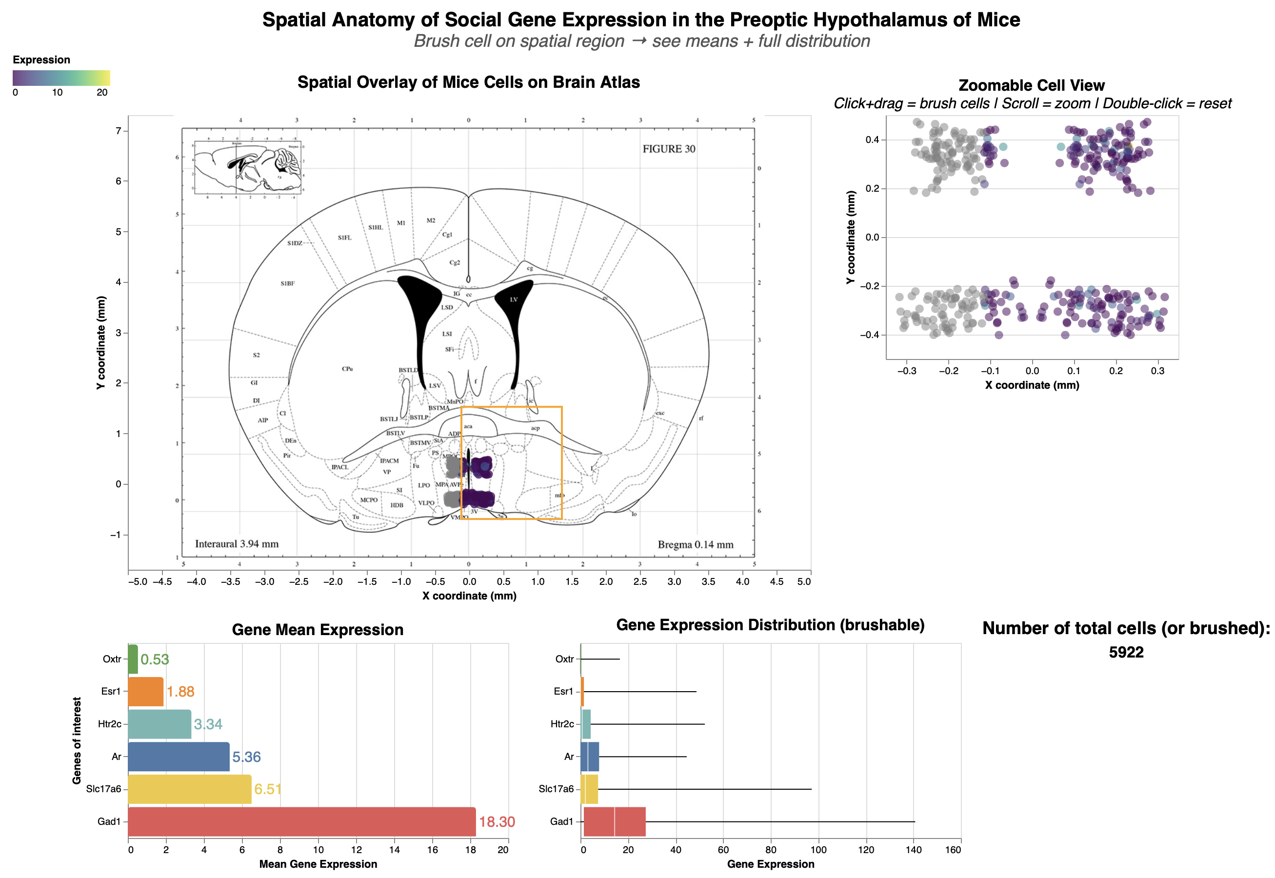
Title: Spatial Anatomy of Social Gene Exoression in the Preoptic Hypothalamus of Mice
Analytic Questions and Tasks: Where are the cells expressing the socially-relevant genes located within the finer-grained anatomy of the preoptic area?
socially-relevant genes (oxytocin Oxtr, estrogen Esr1, testosterone Ar, serotonin Htr2c)
Excitatory signalling marker: Slc17a6
Inhibitory signalling marker: Gad1
Low-Level Tasks Supports
| Visualization / Interaction | Achieved Low-Level Tasks |
|---|---|
| Overlaid Spatial Scatter Plot (Cells on Atlas at Bregma 0.14 mm) |
• Users can identify individual cells by their distinct positions and encodings (e.g., color for gene expression). • Locate enables pinpointing cells relative to atlas landmarks (e.g., sub-regions in the preoptic area). • Cluster reveals perceptual groupings of cells in anatomical regions, helping spot density patterns. |
| Bidirectional Brushing between Overlaid and Non-Overlaid Scatter Plots |
• Brushing allows identifying and locating selected cells at higher resolution in the zoomable plot (overcoming Altair’s overlay limitation). • Supports comparing cell positions/distributions between views and associating selections with linked plots (e.g., updating bar/boxplots), revealing correlations like gene expression variability in brushed regions. |
| Bar Plot (Mean Gene Expression) |
• Bars enable comparing/ranking mean expression levels across genes, with brushing dynamically updating values for selected cells. |
| Boxplot (Gene Expression Distribution) |
• Users compare/rank medians, variability (IQR), and outliers across genes. • Brushing distinguishes distributions for filtered cells and categorizes them by expression levels (e.g., high vs. low variability). |
| Dropdown Filters (Social Behaviors & Specific Genes) |
• Filtering categorizes cells by behaviors or genes, distinguishing subsets (e.g., aggressive vs. nurturing behaviors). |
| Cell Opacity Slider | • Distinguish separates cells from the background atlas via opacity adjustment. |
Encoding, Mark & Channel Description: View I
Encoding:
Scatter plots: The X_coordinate and Y_coordinate attributes correspond the anatomical spatial coordinate for each cell. These two channels were encoded as x and y respectively for the scatter plot.
Bar plot: The x dimension encodes the mean aggregation of expression level, while the y dimension encodes the key social genes.
Scatter plot: The x dimension encodes gene expression level, while the y dimension encodes the key social genes.
Marks: Point (scatter plot), line (bar plot & box plot), area (box plot)
Point was chosen because it marks individual cells as points for showing density and possible clustering spatial pattern.
Line was chosen because the human perception can more reliably perceive difference in line. Mean expression of each gene could be reliably reflected on the aggregated bar chart, and on the box plot, the length of the whisker lines allows user to quickly compare the variability between different genes.
Area in box plot tells us about the precision and variability in one gene around its median over another gene. A smaller box area allows the user to know quickly that this particular gene has uniform expression level close to its medium. Overall, boxplot is a multivariate visual idiom that shows median/IQR/outliers for variability.
Channels: Colour, opacity, position, length
Colous was chosen because it allows quick pre-attentive comparison of the different genes on the bar plot and box plot. The colours were made consistent across the two plot for the same genes.
Opacity was chosen to resolve overplotting problem of the dense cells within the small pre-optic area.
Position: Both positions along the x and y axes were used to express the spatial location of the cells. The vertical position is used for the bar and box plot to list genes of interest.
Length was chosen to represent higher and lower expression level in box and bar plot.
Interactions Description: View I
Bidirectional brushing: Chosen for seamless linking between overlay (brain map) and zoomable scatter plot views. This bidirectional interaction supports:
locate (pinpoint cells in different POA subregions)
cluster (group dense cell patterns via brush)
distinguish (highlight brushed vs. non-brushed points by color/opacity)
compare (contrast expression stats pre/post-brush).
An interested user can brush on different sub-region within the POA to compare expressions of Estrogen vs. Testosteron between different social behaviours.
Dropdowns (filter by behaviour or gene): Selected for categorical cell filtering of different social behaviours and genes. These two dropdowns help with:
categorize (group cells by parenting vs. aggression)
identify (label specific gene expressions)
distinguish/compare (isolate virgin-female vs. male patterns by selecting different dropdown options).
Opacity Slider: Chosen for to balance cell density with atlas visibility and reduce overplotting issue of dense cells. Enables support for:
locate/identify (by lowering the opacity, the brain atlas underneat reveal subregion labels like MPOC (medial preoptic nucleus), MPOM (medial part of medial preoptic), and MPA (medial preoptic) for precise anatomical mapping within the boarder preoptic area.
distinguish (fade cells to show atlas boundaries underneath)
Critique:
The bidirectional brushing on spatial scatters allows direct selection of anatomical cell cluster, which I believe is effective because it dynamically updating bar/box plots for means and variability. Dropdowns filter behaviors/genes, enabling comparisons like Esr1 variability in parenting vs. aggression.
What Works Well: Brushing links anatomy to stats like mean expression level and variability seamlessly, supporting exploratory analysis even for non-experts. Opacity slider aids subregion identification by showing the atlas labelling underneath.
Overplotting was addressed via further downsampling, opacity (alpha) with the opacity slider.
Effective labels & legends: All axes and titles are renamed to nicely formatted names, not just the default attribute names. Different genes were coloured separately.
Visualization Choice: Apt for spatial question—scatters map anatomy directly; bars/boxplots suit summaries/distributions.
Data:Ink Ratio: Used minimal elements (no 3D/backgrounds). I tried improving this aspect by removing redundant color legend for the two scatterplot, which share the same color scheme.
What Could Be Better: Random subsampling from 1 million cells to 10,000 cells was necessary to keep the dashboard responsive, but it would have been more robust if we could include all the cell data. Another huge room for improvement is Altair's disabled zoom on overlays meant that I could not make the brain atlas and scatter overlay zoom-in together. I think this significantly restricts deep dives into examining the anatomical location of the cells.
- Overplotting in the unzoomable scatter-atlas overlay could not be entirely resolved because all the points were densely packed in a small region of the brain. Resolving this issue would require tools beyond Altair unfortuntely.
View II: Expression and co-expression patterns from anterior to posterior part of brain
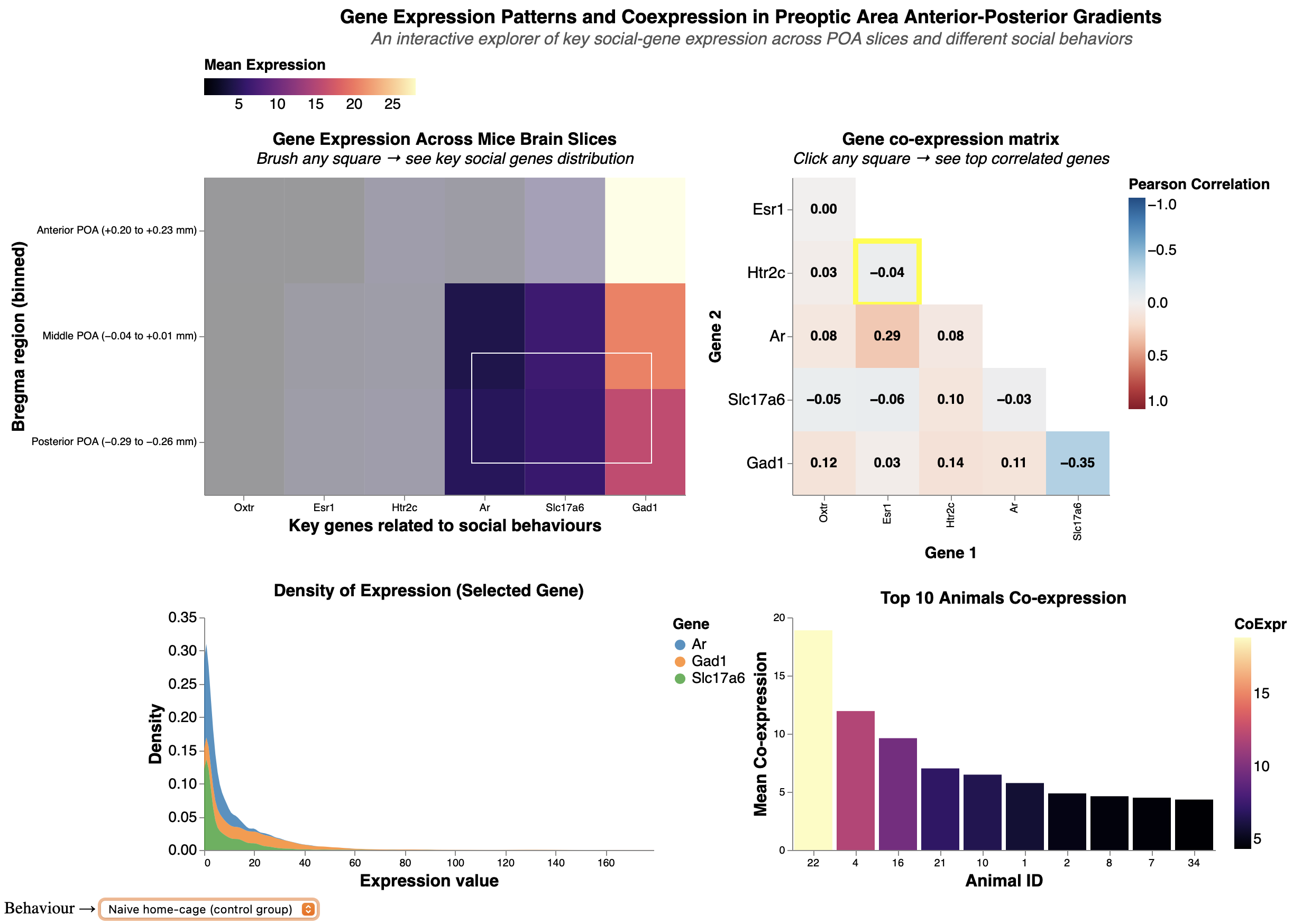
Title: Gene Expression Patterns and Coexpression in Preoptic Area Anterior-Posterior Gradients
Analytic Questions and Tasks: What are the expression densities of key social genes across anterior-middle-posterior POA gradients, and how do pairwise coexpression (correlation) strengths vary by behavior?
For example, testosterone-estrogen (Ar-Esr1) correlation.
Low-Level Tasks Supports
| Visualization / Interaction | Achieved Low-Level Tasks |
|---|---|
| Main Heatmap (Anterior → Posterior POA bins × key genes) |
• Users can rapidly compare and rank gene expression across
anterior–posterior brain positions via the purple → beige gradient. • Identification and distinction of high-expression regions are supported by strong pre-attentive color mapping. • Brushing supports clustering of contiguous high-expression zones. |
| Brushing on the Bregma × Gene Heatmap | • Brushing lets the user identify and locate specific bregma bin & gene combinations, then immediately associate those selections with the expression density plot below. |
| Expression Layered Density Plot (updated by brushing) |
• Multiple overlapping density curves (one per selected gene) allow
direct comparison of distribution shape, median, and spread. • Color encoding by gene supports fast distinction. • Tightly linked to brushed region, revealing how expression variability changes along the anterior–posterior axis or in specific sub-regions. |
| Staircase Gene–Gene Co-expression
Matrix (Pearson r with annotations) |
• The blue–white–red divergent colormap and numerical annotations
enable precise comparison and ranking of co-expression strength
between any gene pair. • Users can identify the strongest positive/negative pairs at a glance and distinguish meaningful correlations from noise. • Directly supports correlation/association tasks at the gene level. |
| Click Interaction on a co-expression matrix cell → Top-10 Animals Bar Chart | • Clicking a correlation cell identifies a specific gene pair
and instantly associates it with the animals that most strongly
exhibit that co-expression pattern. • The ranked bar chart allows users to compare and order animals by co-expression strength and, via tooltips, identify metadata (animal ID, sex). |
| Global Social-Behavior Dropdown (affects all charts in View 2) |
• Instantly categorizes the entire dataset by behavior (e.g., parental vs. aggressive), allowing users to distinguish and compare expression patterns, density distributions, and co-expression strengths between behavioral conditions. |
Mark & Channel Description: View II
Marks: Area (heatmaps, density plot), line (bar plot)
Area was chosen because it marks individual cells as points for showing density and possible clustering spatial pattern.
Line was chosen because the human perception can more reliably perceive difference in line. Mean expression of each gene could be reliably reflected on the aggregated bar chart, and on the box plot, the length of the whisker lines allows user to quickly compare the variability between different genes.
Area in box plot tells us about the precision and variability in one gene around its median over another gene. A smaller box area allows the user to know quickly that this particular gene has uniform expression level close to its medium. Overall, boxplot is a multivariate visual idiom that shows median/IQR/outliers for variability.
Channels: Colour, length, position
Colour - color gradient was chosen to color for the Bregma-Gene heatmap and the Top-10 animals bar chart. The same color gradient scale was used for both of these plots to maintain consistency and reinforces the user's association between "light color = high expression" and "darker color = lower expression" in this View, matching “more ink = more value”.
Gradient is chosen for gene expression level (and its aggregates) because they contain natural order.
Color - color hue was used for the layered density plot to color different genes. Hue was chosen because there is no natural sequential ordering between different genes (nominal).
Length was chosen for representing high (longer length) and low (shorter length) co-expression level between different Top 10 mice. This is to complement color gradient, since our human perception is more sensitive to difference in length than to color gradient.
Position (horizontal) was chosen for representing different genes along the x axis in the heatmaps.
Encoding:
Bregma heatmap: The x dimension encodes different genes, while the y dimension encodes the 3 levels of spatial location (anterior, middle, and posterior brain).
Coexpression heatmap/correlation matrix: Both x and y dimensions encode the same set of key social genes, since the objective of this plot is to look at the correlation between each gene pair.
Layered density plot: The x dimension encodes gene expression level, while the y dimension encodes the density (frequency) of expression level.
Top coexpression animals bar plot: The x dimension encodes for different experimental mice in this data, while the y dimension encodes the mean co-expression of a given gene-pair.
Interactions: View II:
Brushing (on Bregma-gene heatmap): Chosen to dynamically subset gradients, turning 3D (A-M-P bins) into interactive 2D (reduce ink ratio too!). Supports:
cluster (group high-density bins)
distinguish (separate anterior vs. posterior patterns)
locate (position along Bregma)
characterize distribution/compare,
- For example: Brushing to select different anterior and/or posterior part of the brain updates density plot and contrast different social genes.
Clicking (selection_point on coexpression heatmap): Chosen for on-demand selection into gene pairs (e.g., Ar-Esr1 show moderate correlation). Clicking aids:
identify (label pair strengths via Pearson correlation coefficient)
compare (contrast coexpression across genes/behaviors)
Behavior Dropdown (links all views): Mirrors Dashboard 1 for consistency, and it enables:
categorize (by behaviours, like mating vs. parenting mice)
compare (shows behavioral coexpression differences).
Critique:
This view is well-suited for answering: What are the expression densities of key social genes across anterior-middle-posterior POA gradients, and how do pairwise coexpression strengths vary. The heatmaps provide gradient overviews of expression levels and co-expression strength, incorporating brushing/clicking to link the heatmaps to expression distribution (density plot) and animal-specific gene coexpressions. Behavior dropdown ties gene expression patterns to social function.
And based on the course principle, there are aspects of View 2 which is done great and/or need improvements:
Proportional Ink: High-heatmap rects/annotations scale with r/density proportionally; bars reflect true coexpression means. However, it is mildly violated because the x-axis in density plots was truncated due to extreme outlier that flows outside the plot space.
Data:Ink Ratio: Mediocre-color scheme for color gradient was kept consistent. However, I decided to add the correlation coefficients on top of each gene pairs in the coexpression matrix, and I also added an annotation on the side telling the user to click on the matrix. This can be improved by removing the correlation coefficient annotation and rely on just the tooltip popup (which is already there).
Labels & Legends: Clear-axes label are all renamed to avoid defaulting to the attribute names.
Overplotting: The bar plot's width was adjusted so as to not overlap each other. However, the density plots can have further improvement by reducing the overlaps if it is plotted as a ridge plot instead. It can also be bettered with alpha in density or vertically faceted, but faceting will demand more vertical scrolling.
Visualization Choice: Fits gene expression/coexpression query—heatmaps for expression gradient overview, bars for honing in onto separate mouse.
Colour & Accessibility: Color hues were applied to nominal attributes without intrinsic ordering (different genes), while color gradients were applied attributes like expression or its aggregate since they have sequential orders. However, there seems to be too many colors involved in this view, which might be improved by faceting the layered density plot by genes and remove the color channel for the density plot.
Individual Summary
My analysis explores the anatomical locations of cells in the hypothalamic preoptic area (POA) and their gene expressions to get at the overall theme of molecular-spatial-functional organization. Dashboard 1 addresses where cells expressing socially-relevant genes (e.g., Ar, Esr1, Oxtr) are located within finer-grained POA subregions like MPOC, MPOM, and MPA, via spatial overlays and linked stats on means/variability. Dashboard 2 examines expression densities across anterior-middle-posterior gradients and pairwise coexpression strengths (e.g., Ar-Esr1 correlations) varying by behavior, revealing neuromodulatory patterns in social contexts like parenting or aggression.
Successes included robust interactions: bidirectional brushing between spatial scatters enabled seamless subregion selection and gene stats updates, a debugging win that enhanced EDA flow. Dropdowns for behaviors/genes and the opacity slider supported flexible, user-driven comparisons, making the dashboards accessible for non-experts while preserving data fidelity on ~10k subsampled cells.
Challenges arose from Altair limitations, like no zooming on mark_image() overlays, hindering dense cluster inspection despite a separate zoomable scatter. In View 2, color gradients felt overwhelming across heatmaps and densities; faceting or ridge plots could clarify layered distributions but risked vertical space overload, potentially cluttering the view for group use.
Group Summary
Our group investigated brain cell variety, how males and females differ in brain activity, and where cells are situated in the hypothalamic preoptic zone using MERFISH data. We built a flexible dashboard with linked views, allowing users to explore from broad layout cues down to single-cell gene expression.
What ties every theme into one system? This dashboard builds on three linked ideas: spatial and molecular identity, patterns tied to sex-based activity, and a breakdown of variations in the data.
Spatial and Molecular Identity
This part shows how cells are arranged in the preoptic area. One view maps out where different brain cells sit across tissue sections, while another verifies those types by identifying genes such as *Gad1*. Together, they provide a structural and genetic backdrop for the rest of the study.
Sex-Specific Activation
Expanding from the layout map, this section zeroes in on functional activity. Instead of just location, one view displays overall trends, showing where male or female bias pops up during specific actions. Meanwhile, another view pinpoints those active pathways directly onto brain space, allowing users to spot exactly which parts of the foundational structure light up differently by sex.
Variance & Robustness
This component delves into statistical validation to support the findings. One view distinguishes whether observed differences come from sex or from random technical noise like Animal ID. Another view tests if correcting for those batch issues was effective. On top of that, a granular view checks single cells to confirm that patterns make biological sense. So when sex-based gaps are observed in the activation patterns, we know they’re real, not flukes tied to one animal or another.
Overall Takeaways
These visuals team up to expose a layered yet dynamic system. Our findings prove that even though each animal’s unique biology shapes overall gene activity, clear sex-based trends still emerge - especially in hormone-related genes or during specific behaviors like parenting. Location matters: brain circuits favoring one sex aren’t scattered randomly - they are situated within specific zones. Mixing precise maps, real-time brain responses, and solid numerical checks helps scientists unpack how social actions form, shifting from broad clues to trustworthy biological truths. Colors stay uniform, panels connect, and filters sync - all parts talk to each other so users can dive deep without getting lost.